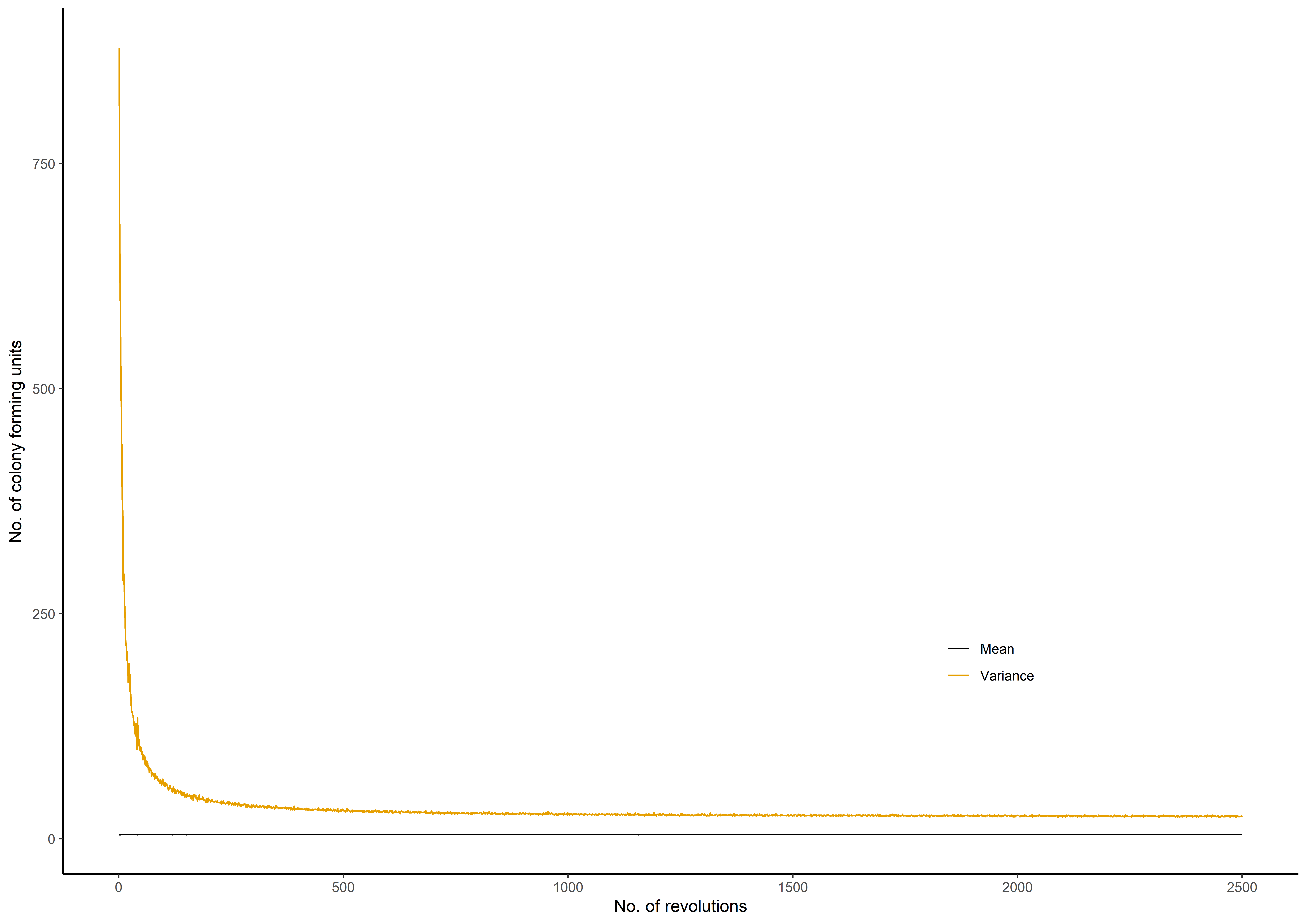
Mean and variance of the expected number of CFUs at each mixing stage.

This function provides the mean and variance of the expected number of CFUs at each mixing stage.

sim_meanvar_stages(mu, sigma, alpha_in, k, l, r, distribution, n_sim)

Arguments

mu

the average number of CFUs (\(\mu\)) in the mixed sample, which is in a logarithmic scale if we use a Lognormal / Poisson lognormal distribution

sigma

the standard deviation of the colony-forming units in the mixed sample on the logarithmic scale (default value 0.8)

alpha_in

concentration parameter at the initial stage

k

number of small portions / primary samples

l

number of revolutions / stages

r

the rate of the concentration parameter changes at each mixing stage

distribution

what suitable distribution type we have employed for simulation such as "Poisson-Type A" or "Poisson-Type B" or "Lognormal-Type A" or "Lognormal-Type B" or "Poisson lognormal-Type A" or "Poisson lognormal-Type B"

n_sim

number of simulations

Value

Mean and variance changes at each mixing stage.

Details

Let \(N'\) be the number of colony-forming units in the mixed sample which is produced by mixing of \(k\) primary samples and \(N' = \sum N_i\). This function produces a graphical display of the mean and variance changes at each mixing stage. It is helpful to identify the optimal number of revolutions of the mixture, which is a point of mixing that initiates Poisson-like homogeneity.

Examples

mu <- 100
sigma <- 0.8
alpha_in <- 0.01
k <- 30
l <- 2500
r <- 0.01
distribution <-  "Poisson lognormal-Type B"
n_sim <- 2000
result1 <- sim_meanvar_stages(mu, sigma , alpha_in, k, l, r, distribution, n_sim)
melten.Prob <- reshape2::melt(result1, id = "Revolutions",
variable.name = "summary", value.name = "Value")
plot_example <- ggplot2::ggplot(melten.Prob, ggplot2::aes(x = Revolutions,
y = Value, group = summary, colour = summary)) +
ggplot2::geom_line(ggplot2::aes(x = Revolutions, y = Value)) +
ggplot2::ylab(expression("No. of colony forming units")) +
ggplot2::theme_classic() + ggplot2::xlab(expression("No. of revolutions")) +
ggplot2::theme(plot.title = ggplot2::element_text(hjust = 0.5),
legend.position = c(0.75,0.25),legend.title = ggplot2::element_blank()) +
ggthemes::scale_colour_colorblind()
plot_example