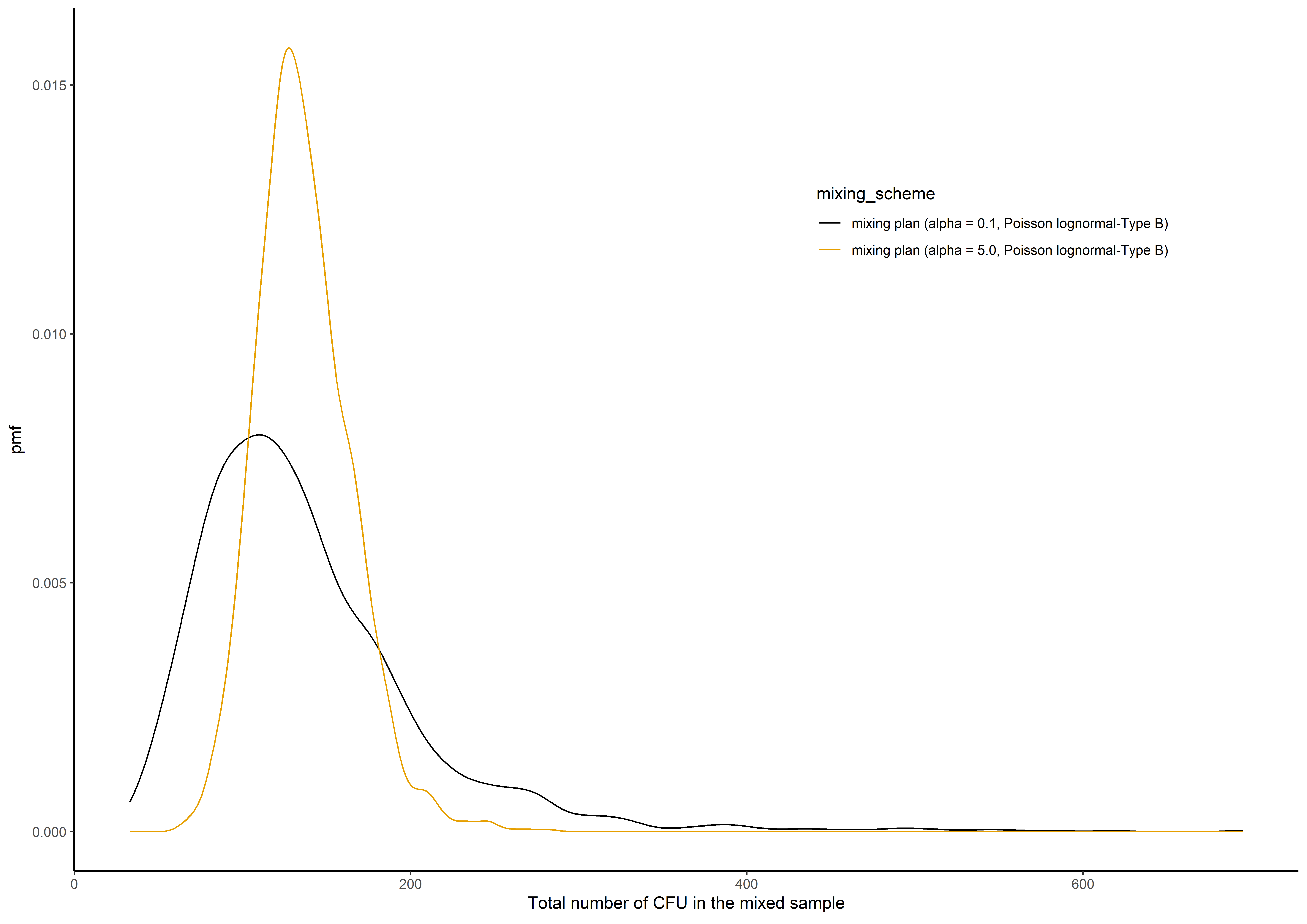
The expected total number of colony-forming units in the mixed sample in the multiple mixing schemes at the single stage of the mixing process.
Source:R/sim_multiple.R
sim_multiple.RdThis function calculates the resulting expected total number of colony-forming units in the mixed sample in the multiple mixing plans at the single stage of the mixing process.
sim_multiple(mu, sigma, alpha, k, distribution, summary, n_sim)Arguments
- mu
the average number of CFUs (\(\mu\)) in the mixed sample, which is in a logarithmic scale if we use a Lognormal / Poisson lognormal distribution
- sigma
the standard deviation of the colony-forming units in the mixed sample on the logarithmic scale (default value 0.8)
- alpha
concentration parameter
- k
number of small portions / primary samples
- distribution
what suitable distribution type we have employed for simulation such as
"Poisson-Type A"or"Poisson-Type B"or"Lognormal-Type A"or"Lognormal-Type B"or"Poisson lognormal-Type A"or"Poisson lognormal-Type B"- summary
if we need to get all simulated \(N'\), use
summary = 2; otherwise, if we usesummary = 1, the function provides the mean value of the simulated \(N'\).- n_sim
number of simulations
Value
total number of colony forming units in the multiple mixing scheme
Details
Let \(N'\) be the number of colony-forming units in the mixed sample which is produced by contribution of \(k\) primary samples mixing and \(N' = \sum N_i\). This function provides the simulated resulting of the expected total number of colony-forming units in the mixed sample in the multiple mixing plans at the single stage of the mixing process. To more details, please refer the details section of compare_mixing_3.
References
Nauta, M.J., 2005. Microbiological risk assessment models for partitioning and mixing during food handling. International Journal of Food Microbiology 100, 311-322.
See also
Examples
set.seed(1350)
mu <- 100
sigma <- 0.8
alpha <- c(0.1,5)
k <- c(30,30)
distribution <-  "Poisson lognormal-Type B"
n_sim <- 2000
f_spri <- function(alpha, distribution) {
sprintf("mixing plan (alpha = %.1f, %s)", alpha, distribution)
}
sim.sum3 <- sim_multiple(mu, sigma, alpha, k, distribution, summary = 2, n_sim)
result <- data.frame(1:n_sim, sim.sum3)
colnames(result) <- c("n_sim", f_spri(alpha, distribution))
melten.Prob <- reshape2::melt(result, id = "n_sim", variable.name = "mixing_scheme",
                              value.name = "Total_CFU")
plot_example <-
ggplot2::ggplot(melten.Prob, ggplot2::aes(Total_CFU, group = mixing_scheme,colour = mixing_scheme))+
ggplot2::geom_line(stat="density",ggplot2::aes(x = Total_CFU))+
ggplot2::ylab(expression("pmf"))+
ggplot2::theme_classic()+ ggplot2::xlab(expression("Total number of CFU in the mixed sample"))+
ggplot2::theme(plot.title = ggplot2::element_text(hjust = 0.5), legend.position = c(0.75,0.75))+
ggthemes::scale_colour_colorblind()
plot_example