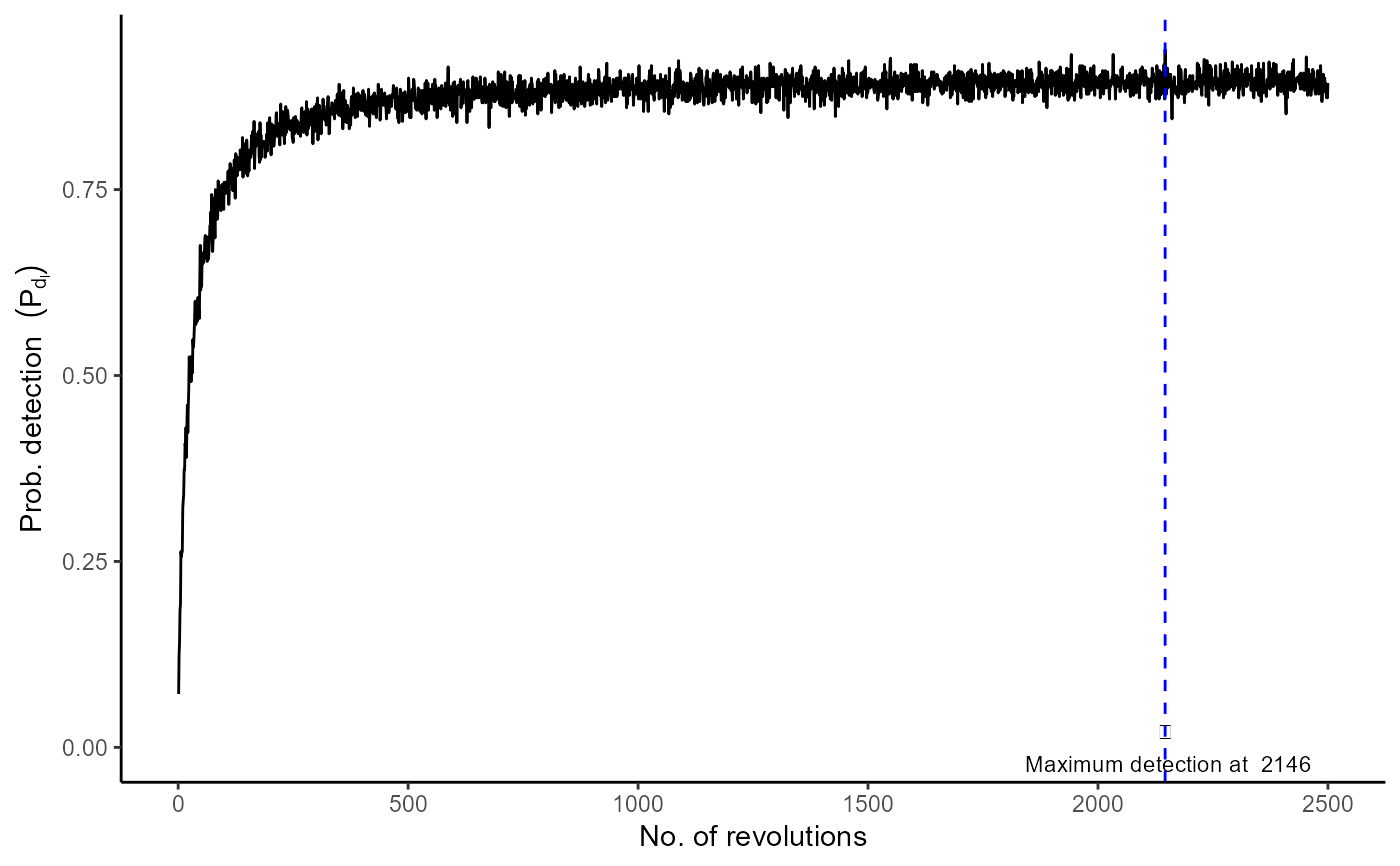
The estimated value of detection probability at each stage (or revolution) of the mixing process.

This function gives a probability of detection at each stage (or revolution) of the mixing process.

sim_single_pd_stages(mu, sigma, alpha_in, k, l, r, distribution, UDL, n_sim)

Arguments

mu: the average number of CFUs (\(\mu\)) in the mixed sample, which is in a logarithmic scale if we use a Lognormal / Poisson lognormal distribution
sigma: the standard deviation of the colony-forming units in the mixed sample on the logarithmic scale (default value 0.8)
alpha_in: concentration parameter at the initial stage
k: number of small portions / primary samples
l: number of revolutions /stages
r: the rate of the concentration parameter changes at each mixing stage
distribution: what suitable distribution type we have employed for simulation such as "Poisson-Type A" or "Poisson-Type B" or "Lognormal-Type A" or "Lognormal-Type B" or "Poisson lognormal-Type A" or "Poisson lognormal-Type B"
UDL: the upper decision limit, which depends on the type of microorganisms and testing regulations.
n_sim: number of simulations

Value

The probability of detection at each stage of the mixing process.

Details

Let \(N'\) be the number of CFUs in the mixed sample, which is produced by the contribution of \(k\) primary samples mixing, \(N' = \sum N_i\) and let \(l\) be the number of stages in the mixing process. This function provides probability of detection at each stage of the mixing process. At each stage (or revolution), the probability of detection (\(p_d\)) can be estimated by using function sim_single_pd.

References

Nauta, M.J., 2005. Microbiological risk assessment models for partitioning and mixing during food handling. International Journal of Food Microbiology 100, 311-322.

Examples

mu <- 100
sigma <- 0.8
alpha_in <- 0.01
k <- 30
l <- 2500
r <- 0.01
distribution <- "Poisson lognormal-Type B"
UDL <- 0
n_sim <- 20
stages <- c(1:l)
Prob_df <-
data.frame(stages,sim_single_pd_stages(mu,sigma,alpha_in,k,l,r,distribution,UDL,n_sim))
colnames(Prob_df) <- c("no.revolutions","prob.detection")
plot_example <- ggplot2::ggplot(Prob_df) +
ggplot2::geom_line(ggplot2::aes(x = stages, y = prob.detection)) +
#ggplot2::stat_smooth(geom = "smooth", method = "gam", mapping = ggplot2::aes(x = no.revolutions,
#y = prob.detection), se = FALSE, n = 1000) +
ggplot2::ylab(expression("Prob. detection" ~~ (P[d[l]]))) +
ggplot2::theme_classic() + ggplot2::xlab(expression("No. of revolutions")) +
ggplot2::theme(plot.title = ggplot2::element_text(hjust = 0.5), legend.position = c(0.75,0.25)) +
#ggplot2::ggtitle(label = f_spr(n_sim))+
ggplot2::geom_vline(xintercept = which.max(Prob_df$prob.detection),
linetype = "dashed",colour = "blue") +
ggplot2::annotate("text", x = which.max(Prob_df$prob.detection), y = 0,
label = sprintf("\n Maximum detection at  %0.0f",round(which.max(Prob_df$prob.detection)))
, size = 3)+
ggthemes::scale_colour_colorblind()
print(plot_example)